Analyzing Molecular Data

Overview

Teaching: 40 min
Exercises: 20 min

Questions

• How can I process tabular data files in Python?

Objectives

• Explain what a library is and what libraries are used for.

• Import a Python library and use the functions it contains.

• Read tabular data from a file into a program.

• Select individual values and subsections from data.

• Perform operations on arrays of data.

Words are useful, but what’s more useful are the sentences and stories we build with them. Similarly, while a lot of powerful, general tools are built into Python, specialized tools built up from these basic units live in libraries that can be called upon when needed.

Loading data into Python

To begin processing inflammation data, we need to load it into Python. We can do that using a library called NumPy, which stands for Numerical Python. In general, you should use this library when you want to do fancy things with lots of numbers, especially if you have matrices or arrays. To tell Python that we’d like to start using NumPy, we need to import it:

import numpy

Importing a library is like getting a piece of lab equipment out of a storage locker and setting it up on the bench. Libraries provide additional functionality to the basic Python package, much like a new piece of equipment adds functionality to a lab space. Just like in the lab, importing too many libraries can sometimes complicate and slow down your programs - so we only import what we need for each program.

Once we’ve imported the library, we can ask the library to read our data file for us:

numpy.loadtxt(fname='combined-no-headers.csv', delimiter=',')

array([[ 0.00000000e+00  6.00000000e+00 -9.00000000e-02 ...  2.02559852e+01
   2.79454641e+02  1.00000000e+00]
 [ 1.00000000e+00  2.33333333e+00 -9.00000000e-02 ...  2.02559852e+01
   2.79454641e+02  1.00000000e+00]
 [ 2.00000000e+00  7.90000000e+01 -1.40000000e-01 ...  7.60741678e+01
   2.23068184e+02  5.00000000e-01]
 ...
 [ 3.40000000e+02  2.00000000e+00  3.60000000e-01 ...  8.45799261e+01
   3.94431707e+02  5.00000000e-01]
 [ 3.41000000e+02  1.50000000e+01  3.60000000e-01 ...  8.45799261e+01
   2.82386669e+02  5.00000000e-01]
 [ 3.42000000e+02  3.00000000e-01  0.00000000e+00 ...  8.45799261e+01
   2.43000629e+02  5.00000000e-01]])

The expression numpy.loadtxt(...) is a function call that asks Python to run the function loadtxt which belongs to the numpy library. This dotted notation is used everywhere in Python: the thing that appears before the dot contains the thing that appears after.

As an example, John Smith is the John that belongs to the Smith family. We could use the dot notation to write his name smith.john, just as loadtxt is a function that belongs to the numpy library.

numpy.loadtxt has two parameters: the name of the file we want to read and the delimiter that separates values on a line. These both need to be character strings (or strings for short), so we put them in quotes.

Since we haven’t told it to do anything else with the function’s output, the notebook displays it. In this case, that output is the data we just loaded. By default, only a few rows and columns are shown (with ... to omit elements when displaying big arrays). Note that, to save space when displaying NumPy arrays, Python does not show us trailing zeros, so 1.0 becomes 1..

Our call to numpy.loadtxt read our file but didn’t save the data in memory. To do that, we need to assign the array to a variable. In a similar manner to how we assign a single value to a variable, we can also assign an array of values to a variable using the same syntax. Let’s re-run numpy.loadtxt and save the returned data:

data = numpy.loadtxt(fname='combined-no-headers.csv', delimiter=',')

This statement doesn’t produce any output because we’ve assigned the output to the variable data. If we want to check that the data have been loaded, we can print the variable’s value:

print(data)

[[ 0.00000000e+00  6.00000000e+00 -9.00000000e-02 ...  2.02559852e+01
   2.79454641e+02  1.00000000e+00]
 [ 1.00000000e+00  2.33333333e+00 -9.00000000e-02 ...  2.02559852e+01
   2.79454641e+02  1.00000000e+00]
 [ 2.00000000e+00  7.90000000e+01 -1.40000000e-01 ...  7.60741678e+01
   2.23068184e+02  5.00000000e-01]
 ...
 [ 3.40000000e+02  2.00000000e+00  3.60000000e-01 ...  8.45799261e+01
   3.94431707e+02  5.00000000e-01]
 [ 3.41000000e+02  1.50000000e+01  3.60000000e-01 ...  8.45799261e+01
   2.82386669e+02  5.00000000e-01]
 [ 3.42000000e+02  3.00000000e-01  0.00000000e+00 ...  8.45799261e+01
   2.43000629e+02  5.00000000e-01]]

Now that the data are in memory, we can manipulate them. First, let’s ask what type of thing data refers to:

print(type(data))

<class 'numpy.ndarray'>

The output tells us that data currently refers to an N-dimensional array, the functionality for which is provided by the NumPy library. These data correspond to arthritis patients’ inflammation. The rows are the individual patients, and the columns are their daily inflammation measurements.

Data Type

A Numpy array contains one or more elements of the same type. The type function will only tell you that a variable is a NumPy array but won’t tell you the type of thing inside the array. We can find out the type of the data contained in the NumPy array.

print(data.dtype)

float64

This tells us that the NumPy array’s elements are floating-point numbers.

With the following command, we can see the array’s shape:

print(data.shape)

(343, 23)

The output tells us that the data array variable contains 343 rows and 23 columns. When we created the variable data to store our arthritis data, we did not only create the array; we also created information about the array, called members or attributes. This extra information describes data in the same way an adjective describes a noun. data.shape is an attribute of data which describes the dimensions of data. We use the same dotted notation for the attributes of variables that we use for the functions in libraries because they have the same part-and-whole relationship.

If we want to get a single number from the array, we must provide an index in square brackets after the variable name, just as we do in math when referring to an element of a matrix. Our molecular properties data has two dimensions, so we will need to use two indices to refer to one specific value:

print('first value in data:', data[0, 0])

first value in data: 0.0

print('middle value in data:', data[172, 11])

middle value in data: 94.18429025

The expression data[172, 11] accesses the element at row 172, column 11. While this expression may not surprise you, data[0, 0] might. Programming languages like Fortran, MATLAB and R start counting at 1 because that’s what human beings have done for thousands of years. Languages in the C family (including C++, Java, Perl, and Python) count from 0 because it represents an offset from the first value in the array (the second value is offset by one index from the first value). This is closer to the way that computers represent arrays (if you are interested in the historical reasons behind counting indices from zero, you can read Mike Hoye’s blog post). As a result, if we have an M×N array in Python, its indices go from 0 to M-1 on the first axis and 0 to N-1 on the second. It takes a bit of getting used to, but one way to remember the rule is that the index is how many steps we have to take from the start to get the item we want.

In the Corner

What may also surprise you is that when Python displays an array, it shows the element with index [0, 0] in the upper left corner rather than the lower left. This is consistent with the way mathematicians draw matrices but different from the Cartesian coordinates. The indices are (row, column) instead of (column, row) for the same reason, which can be confusing when plotting data.

Slicing data

An index like [30, 20] selects a single element of an array, but we can select whole sections as well. For example, we can select the first properties (columns) of values for the first four molecules (rows) like this:

print(data[0:4, 0:10])

[[ 0.00000000e+00  6.00000000e+00 -9.00000000e-02  0.00000000e+00
   0.00000000e+00 -9.00000000e-02  0.00000000e+00  0.00000000e+00
   0.00000000e+00  0.00000000e+00]
 [ 1.00000000e+00  2.33333333e+00 -9.00000000e-02  0.00000000e+00
   0.00000000e+00 -9.00000000e-02  0.00000000e+00  0.00000000e+00
   0.00000000e+00  0.00000000e+00]
 [ 2.00000000e+00  7.90000000e+01 -1.40000000e-01  0.00000000e+00
   0.00000000e+00  0.00000000e+00 -1.70000000e-01  0.00000000e+00
  -2.70000000e-01  0.00000000e+00]
 [ 3.00000000e+00  9.75000000e+01  7.00000000e-02  0.00000000e+00
   0.00000000e+00 -1.20000000e-01 -1.70000000e-01  0.00000000e+00
  -2.70000000e-01  0.00000000e+00]]

The slice 0:4 means, “Start at index 0 and go up to, but not including, index 4”. Again, the up-to-but-not-including takes a bit of getting used to, but the rule is that the difference between the upper and lower bounds is the number of values in the slice.

We don’t have to start slices at 0:

print(data[5:10, 0:10])

[[ 5.000e+00  9.575e+01  0.000e+00  0.000e+00  0.000e+00  0.000e+00
  -1.700e-01  0.000e+00 -2.700e-01  0.000e+00]
 [ 6.000e+00  9.650e+01 -1.600e-01  0.000e+00  0.000e+00 -1.000e-02
  -1.700e-01  0.000e+00 -2.700e-01  0.000e+00]
 [ 7.000e+00  9.400e+01 -9.000e-02  0.000e+00  0.000e+00 -1.000e-02
  -1.700e-01  0.000e+00 -2.700e-01  0.000e+00]
 [ 8.000e+00  1.250e+00  0.000e+00  0.000e+00  0.000e+00 -1.700e-01
   0.000e+00  0.000e+00 -1.500e-01  0.000e+00]
 [ 9.000e+00  2.250e+00 -9.000e-02  0.000e+00  0.000e+00 -9.000e-02
   0.000e+00  0.000e+00  0.000e+00  1.000e+00]]

We also don’t have to include the upper and lower bound on the slice. If we don’t include the lower bound, Python uses 0 by default; if we don’t include the upper, the slice runs to the end of the axis, and if we don’t include either (i.e., if we use ‘:’ on its own), the slice includes everything:

small = data[:3, 18:]
print('small is:')
print(small)

The above example selects rows 0 through 2 and columns 36 through to the end of the array.

small is:
[[  0.           0.          20.25598522 279.4546413    1.        ]
 [  0.           0.          20.25598522 279.4546413    1.        ]
 [ 21.5742147    0.          76.07416785 223.0681843    0.5       ]]

Analyzing data

NumPy has several useful functions that take an array as input to perform operations on its values. If we want to find the average inflammation for all patients on all days, for example, we can ask NumPy to compute data’s mean value:

Let’s first remove the first column, our data lables which have been interpreted as real numbers

data = np.delete(data, 0, 1)

And now we can compute the mean

print(numpy.mean(data))

53.72029602831553

mean is a function that takes an array as an argument.

Not All Functions Have Input

Generally, a function uses inputs to produce outputs. However, some functions produce outputs without needing any input. For example, checking the current time doesn’t require any input.

import time
print(time.ctime())

Sat Mar 26 13:07:33 2016

For functions that don’t take in any arguments, we still need parentheses (()) to tell Python to go and do something for us.

Let’s use three other NumPy functions to get some descriptive values about the dataset. We’ll also use multiple assignment, a convenient Python feature that will enable us to do this all in one line.

maxval, minval, stdval = numpy.max(data), numpy.min(data), numpy.std(data)

print('maximum property:', maxval)
print('minimum property:', minval)
print('standard deviation:', stdval)

Here we’ve assigned the return value from numpy.max(data) to the variable maxval, the value from numpy.min(data) to minval, and so on.

maximum property: 646.1013477
minimum property: -0.27
standard deviation: 98.0360663022302

Mystery Functions in IPython

How did we know what functions NumPy has and how to use them? If you are working in IPython or in a Jupyter Notebook, there is an easy way to find out. If you type the name of something followed by a dot, then you can use tab completion (e.g. type numpy. and then press Tab) to see a list of all functions and attributes that you can use. After selecting one, you can also add a question mark (e.g. numpy.cumprod?), and IPython will return an explanation of the method! This is the same as doing help(numpy.cumprod). Similarly, if you are using the “plain vanilla” Python interpreter, you can type numpy. and press the Tab key twice for a listing of what is available. You can then use the help() function to see an explanation of the function you’re interested in, for example: help(numpy.cumprod).

When analyzing data, though, we often want to look at variations in statistical values, such as the maximum feature per molcule or the average of a feature across all molecules. One way to do this is to create a new temporary array of the data we want, then ask it to do the calculation:

molecule_0 = data[0, :] # 0 on the first axis (rows), everything on the second (columns)
print('maximum property for molecule 0:', numpy.max(patient_0))

maximum property for molecule 0: 279.4546413

Everything in a line of code following the ‘#’ symbol is a comment that is ignored by Python. Comments allow programmers to leave explanatory notes for other programmers or their future selves.

We don’t actually need to store the row in a variable of its own. Instead, we can combine the selection and the function call:

print('maximum feature for molecule 2:', numpy.max(data[2, :]))

maximum feature value for molecule 2: 223.0681843

What if we need the maximum feature value for each molecule (as in the next diagram on the left) or the average for each feature over all molecules(as in the diagram on the right)? As the diagram below shows, we want to perform the operation across an axis:

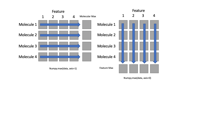
To support this functionality, most array functions allow us to specify the axis we want to work on. If we ask for the average across axis 0 (rows in our 2D example), we get:

print(numpy.mean(data, axis=0))

[ 3.08195303e+01  2.47230321e-02 -2.65597668e-02 -1.11370262e-02
 -2.74344023e-02 -4.00874636e-02 -1.54810496e-02 -1.09766764e-01
  5.18950437e-01  3.00224099e+02  7.87582274e+01  1.38170875e+02
  1.38170875e+02  6.06081019e+00  1.13154699e+01  3.23403644e+01
  5.94126474e+01  7.38168047e+00  2.10248945e+01  5.16751691e+01
  3.05429392e+02  7.49271137e-01]

As a quick check, we can ask this array what its shape is:

print(numpy.mean(data, axis=0).shape)

(22,)

The expression (22,) tells us we have an N×1 vector, so this is the average for each feature for all patients. If we average across axis 1 (columns in our 2D example), we get:

print(numpy.mean(data, axis=1))

[51.99058494 51.82391827 34.7444164  47.51821009 53.10204261 46.88745401
 56.56150193 62.33442536 36.76296138 51.86558494 51.93376676 51.87694857
 51.99058494 51.96785766 51.99058494 52.39967585 48.50888887 51.17339899
 52.51430808 51.53703536 51.07226263 51.09764142 51.09006566 51.11279293
 51.09385354 51.07112626 51.10521717 51.05976263 51.05976263 51.03703536
 51.0824899  51.09385354 51.01430808 51.12794445 52.15067172 59.09881634
 59.62154362 81.7668866  84.71718103 85.35354466 64.65989297 70.35633877
 64.69777176 47.56366464 36.79705229 43.97138102 46.05687761 53.92547678
 65.19569877 58.29873336 61.52907595 25.90992692 38.79831223 47.22487446
 47.56474037 29.25618039 36.74523411 33.06116179 40.50612461 35.00590436
 64.65231721 64.65231721 64.72049903 64.62958994 64.76595358 64.60686267
 64.77731721 65.83413539 55.04347299 56.08892754 70.52307229 70.40375411
 70.50602684 70.42648138 70.44920865 70.47193593 70.58557229 70.42193593
 70.48329956 70.37193593 70.85829956 70.4946632  70.40375411 70.38102684
 70.44920865 70.72761774 37.86605323 54.08456769 40.9980353  65.28660787
 42.40487934 67.48111633 68.29929815 40.97894439 58.73055154 49.87170881
 61.48362141 54.46929089 45.68393372 42.80692601 48.66797978 45.77484281
 43.97138102 48.75888887 48.69070705 74.68138246 74.65865519 74.77229156
 74.68138246 74.74956428 78.61320065 78.65865519 78.77229156 78.54501883
 78.59047337 78.61320065 78.59047337 46.09096852 46.00005943 46.06824125
 45.69011424 45.71238697 39.69894439 46.0227867  46.06824125 46.04551397
 46.36369579 46.15915034 46.28415034 46.06824125 46.11369579 46.13642306
 46.0227867  46.00005943 46.00005943 46.00005943 46.0227867  46.06824125
 46.03415034 46.0227867  46.0227867  50.47733215 46.09096852 47.00005943
 46.09096852 46.11369579 46.04551397 46.06824125 46.30687761 46.10233215
 46.06824125 46.11369579 46.0227867  46.11369579 46.06824125 46.06824125
 46.06824125 46.70460488 46.00005943 46.0227867  46.06824125 46.04551397
 46.00005943 46.0227867  46.04551397 46.00005943 46.00005943 46.68187761
 47.11369579 73.67545405 86.82517217 53.60184042 53.60184042 53.73820405
 53.69274951 53.69274951 53.67002223 53.73820405 53.64729496 53.62456769
 53.85184042 53.77002223 53.82911314 53.69274951 54.32911314 53.71547678
 49.2855413  49.26281403 49.21735948 49.33099585 49.26281403 49.17190494
 49.33099585 49.21735948 49.19463221 49.05826857 50.79240942 51.5651367
 51.90604579 50.8151367  50.8151367  50.88331851 50.79240942 50.79240942
 50.79240942 63.03017427 89.04005178 89.10823359 44.67502991 89.06277905
 89.13096087 88.62524944 23.94910859 54.63289747 59.27904479 61.31193575
 68.90962583 80.16916601 73.51560969 76.52277046 99.19594174 98.01204849
 27.78408999 50.54895434 25.83445497 48.76477387 48.50888887 40.86076257
 49.68989063 46.25807245 50.52622706 50.79240942 88.99459723 50.59440888
 50.82168161 51.17339899 42.71601692 64.66241822 43.9941083  43.92592648
 43.7441083  43.90319921 47.86825334 47.27734425 47.61825334 25.79629055
 47.56366464 57.69435517 47.45002827 47.427301   47.40457373 47.427301
 56.77609633 56.57155087 47.54093736 36.75159775 47.56366464 38.23657776
 38.21385049 44.03956284 38.21385049 38.32748685 42.30475958 42.19112321
 38.66194859 36.72432502 53.33762084 53.24671175 53.2921663  53.31489357
 53.33762084 53.2921663  53.33762084 53.2921663  53.26943903 53.2921663
 53.31489357 53.26943903 53.33762084 53.31489357 53.31489357 53.32625721
 53.31489357 53.31489357 53.36034812 53.33762084 53.2921663  42.87871884
 42.21962793 43.85599157 53.96748921 51.74058494 36.76523411 37.29705229
 44.00547193 67.5038436  36.74705229 38.19112321 51.83149403 64.60686267
 51.78603948 51.87694857 51.80876676 36.77432502 44.03956284 36.91523411
 36.75159775 41.18341593 41.11523411 41.16068865 36.75159775 51.78603948
 43.92592648 36.77432502 43.51683557 36.81977956 51.80876676 46.92941991
 48.59979796 57.51253699 61.73980971 51.80876676 36.71977956 54.30136226
 51.78129472 51.98198261 72.39885502 72.30794593 72.30794593 72.37612775
 72.35340048 72.48976411 72.33067321 71.62361426 71.64634153 71.73725062
 71.73725062 71.69179607 71.72588698 71.80543244 71.6690688  47.11114202
 36.71977956]

which is the average of all features per molecule.

Slicing Strings

A section of an array is called a slice. We can take slices of character strings as well:

element = 'oxygen'
print('first three characters:', element[0:3])
print('last three characters:', element[3:6])

first three characters: oxy
last three characters: gen

What is the value of element[:4]? What about element[4:]? Or element[:]?

Solution

oxyg
en
oxygen

What is element[-1]? What is element[-2]?

Solution

n
e

Given those answers, explain what element[1:-1] does.

Solution

Creates a substring from index 1 up to (not including) the final index, effectively removing the first and last letters from ‘oxygen’

How can we rewrite the slice for getting the last three characters of element, so that it works even if we assign a different string to element? Test your solution with the following strings: carpentry, clone, hi.

Solution

element = 'oxygen'
print('last three characters:', element[-3:])
element = 'carpentry'
print('last three characters:', element[-3:])
element = 'clone'
print('last three characters:', element[-3:])
element = 'hi'
print('last three characters:', element[-3:])

last three characters: gen
last three characters: try
last three characters: one
last three characters: hi

Thin Slices

The expression element[3:3] produces an empty string, i.e., a string that contains no characters. If data holds our array of patient data, what does data[3:3, 4:4] produce? What about data[3:3, :]?

Solution

array([], shape=(0, 0), dtype=float64)
array([], shape=(0, 22), dtype=float64)

Stacking Arrays

Arrays can be concatenated and stacked on top of one another, using NumPy’s vstack and hstack functions for vertical and horizontal stacking, respectively.

import numpy

A = numpy.array([[1,2,3], [4,5,6], [7, 8, 9]])
print('A = ')
print(A)

B = numpy.hstack([A, A])
print('B = ')
print(B)

C = numpy.vstack([A, A])
print('C = ')
print(C)

A =
[[1 2 3]
 [4 5 6]
 [7 8 9]]
B =
[[1 2 3 1 2 3]
 [4 5 6 4 5 6]
 [7 8 9 7 8 9]]
C =
[[1 2 3]
 [4 5 6]
 [7 8 9]
 [1 2 3]
 [4 5 6]
 [7 8 9]]

Write some additional code that slices the first and last columns of A, and stacks them into a 3x2 array. Make sure to print the results to verify your solution.

Solution

A ‘gotcha’ with array indexing is that singleton dimensions are dropped by default. That means A[:, 0] is a one dimensional array, which won’t stack as desired. To preserve singleton dimensions, the index itself can be a slice or array. For example, A[:, :1] returns a two dimensional array with one singleton dimension (i.e. a column vector).

D = numpy.hstack((A[:, :1], A[:, -1:]))
print('D = ')
print(D)

D =
[[1 3]
 [4 6]
 [7 9]]

Solution

An alternative way to achieve the same result is to use Numpy’s delete function to remove the second column of A.

D = numpy.delete(A, 1, 1)
print('D = ')
print(D)

D =
[[1 3]
 [4 6]
 [7 9]]

Change In Values

Let’s presume for a moment that the data for each molecule is logitudinal in nature. So each value is part of a series over time. We might be interested in the change in that value over time. Let’s find out how to calculate changes in the data contained in an array with NumPy.

The numpy.diff() function takes an array and returns the differences between two successive values. Let’s use it to examine the changes each day across the first week of patient 3 from our inflammation dataset.

molecule3_first7features = data[3, :7]
print(molecule3_first7features)

 [79.   -0.14  0.    0.    0.   -0.17  0.  ]

Calling numpy.diff(molecule3_first7features) would do the following calculations

[-0.14 - 79, 0 - -0.14, 0 - 0, 0 - 0, -0.17 - 0, 0 - -0.17]

and return the 6 difference values in a new array.

numpy.diff(molecule3_first7features)

array([-79.14   0.14   0.     0.    -0.17   0.17])

Note that the array of differences is shorter by one element (length 6).

Key Points

• Import a library into a program using import libraryname.

• Use the numpy and pandas library to work with arrays in Python.

• The expression array.shape gives the shape of an array.

• Use array[x, y] to select a single element from a 2D array.

• Array indices start at 0, not 1.

• Use low:high to specify a slice that includes the indices from low to high-1.

• Use # some kind of explanation to add comments to programs.

• Use numpy.mean(array), numpy.max(array), and numpy.min(array) to calculate simple statistics.

• Use numpy.mean(array, axis=0) or numpy.mean(array, axis=1) to calculate statistics across the specified axis.